Search This Blog

Sunday, 1 September 2019

Spark Memory Management


 Spark’s performance advantage over MapReduce  is due to Spark’s In-Memory Persistence and Memory Management Rather than writing to disk between each pass through the data, Spark has the option of keeping the data on the executors loaded into memory. That way, the data on each partition is available in-memory each time it needs to be accessed.

Spark offers three options for memory management: in-memory as deserialized data, in-memory as serialized data, and on disk. Each has different space and time advantages:


  1. In memory as deserialized Java objects
  2. As serialized data
  3. On disk


In memory as deserialized Java objects
The most intuitive way to store objects in RDDs is as the original deserialized Java objects that are defined by the driver program. This form of in-memory storage is the fastest since it reduces serialization time; however, it may not be the most memory efficient, since it requires the data to be stored as objects.

As serialized data
Spark objects are converted into streams of bytes as they are moved around the network using the standard Java serialization library. This approach may be slower since serialized data is more CPU-intensive to read than deserialized data,
but it is more memory efficient, since it allows the user to choose a more efficient representation. While Java serialization is more efficient than full objects, Kryo serialization can be much better than the java serialization

On disk:

RDDs, whose partitions are too large to be stored in RAM on each of the executors, can be written to disk. This strategy is obviously slower for repeated computations but can be more fault-tolerant for long sequences of transformations, and maybe the only feasible option for enormous computations.

The persist() function in the RDD class lets the user control how the RDD is stored. By default, persist() stores an RDD as deserialized objects in memory, but the user can pass one of nthe umerous storage options to the persist() function to control how the RDD is stored. We will cover the different options for RDD reuse
   “Types of RDD Reuse: Cache, Persist, Checkpoint, Shuffle Files” . When persisting RDDs, the default implementation of RDDs evicts the least recently used partition (called LRU caching) if the space it takes is required to compute or to cache a new partition. However, you can change this behavior and control Spark’s memory prioritization with the persistencePriority() function in the RDD class.

Tuesday, 27 August 2019

Critical Spark Enhancements


Spark is super-slow for all wide data (when there are >15kb columns and >15kb rows). Most of the genomics/transcriptomic data is wide because number of genes is usually >20kb and number of samples ass well. Very popular GTEX dataset is a good example ( see for instance RNA-Seq data athttps://storage.googleapis.com/gtex_analysis_v7/rna_seq_datawhere gct is just a .tsv file with two comments in the beginning). Everything done in wide tables (even simple "describe" functions applied to all the genes-columns) either takes hours or gets frozen (because of lost executors) irrespective of memory and numbers of cores. While the same operations work fast (minutes) and well with pure pandas (without any spark involved). 

https://issues.apache.org/jira/browse/SPARK-28547

Sunday, 23 December 2018

scd type 2 in hive


truncate table cust_income;
truncate table cust_income_intmdt;
truncate table cust_income_target;


insert into table cust_income values
(1,'P','100000','20000','120000','1-2-2016'),
(2,'P','120000','20000','140000','1-2-2016'),
(3,'P','130000','20000','150000','1-2-2016');


insert into cust_income_intmdt
select x.cust_id, x.person_org_code, x.annual_net_inc, x.total_tax, x.est_gross_inc, x.dw_ld_ts, x.start_dt, x.end_dt from cust_income_target x where end_dt is not null
union all
select x.cust_id, x.person_org_code, x.annual_net_inc, x.total_tax, x.est_gross_inc, x.dw_ld_ts, x.start_dt, y.dw_ld_ts end_dt from cust_income_target x
left outer join
cust_income y on (x.cust_id = y.cust_id) where x.end_dt is null
union all
select x.cust_id, x.person_org_code, x.annual_net_inc, x.total_tax, x.est_gross_inc, x.dw_ld_ts, x.dw_ld_ts start_dt, null end_dt from cust_income x ;

truncate table cust_income_target;

insert into cust_income_target
select * from cust_income_intmdt;

truncate table cust_income_intmdt;

truncate table cust_income;

insert into table cust_income values
(1,'P','110000','20000','120000','2-2-2016'),
(2,'P','130000','20000','140000','2-2-2016'),
(4,'P','130000','20000','150000','2-2-2016');

insert into cust_income_intmdt
select x.cust_id, x.person_org_code, x.annual_net_inc, x.total_tax, x.est_gross_inc, x.dw_ld_ts, x.start_dt, x.end_dt from cust_income_target x where end_dt is not null
union all
select x.cust_id, x.person_org_code, x.annual_net_inc, x.total_tax, x.est_gross_inc, x.dw_ld_ts, x.start_dt, y.dw_ld_ts end_dt from cust_income_target x
left outer join
cust_income y on (x.cust_id = y.cust_id) where x.end_dt is null
union all
select x.cust_id, x.person_org_code, x.annual_net_inc, x.total_tax, x.est_gross_inc, x.dw_ld_ts, x.dw_ld_ts start_dt, null end_dt from cust_income x ;

truncate table cust_income_target;

insert into cust_income_target
select * from cust_income_intmdt;

truncate table cust_income_intmdt;

truncate table cust_income;

insert into table cust_income values
(4,'P','120000','20000','120000','3-2-2016'),
(2,'P','140000','20000','140000','3-2-2016'),
(5,'P','150000','20000','150000','3-2-2016');

insert into cust_income_intmdt
select x.cust_id, x.person_org_code, x.annual_net_inc, x.total_tax, x.est_gross_inc, x.dw_ld_ts, x.start_dt, x.end_dt from cust_income_target x where end_dt is not null
union all
select x.cust_id, x.person_org_code, x.annual_net_inc, x.total_tax, x.est_gross_inc, x.dw_ld_ts, x.start_dt, y.dw_ld_ts end_dt from cust_income_target x
left outer join
cust_income y on (x.cust_id = y.cust_id) where x.end_dt is null
union all
select x.cust_id, x.person_org_code, x.annual_net_inc, x.total_tax, x.est_gross_inc, x.dw_ld_ts, x.dw_ld_ts start_dt, null end_dt from cust_income x ;

truncate table cust_income_target;

insert into cust_income_target
select * from cust_income_intmdt;

truncate table cust_income_intmdt;

Monday, 13 November 2017

Abinitio on unix to sqlserver on windows conn requirements

                    Abinitio on unix to sqlserver on windows conn requirements

This article details the steps required to connect from abinitio on linux ot sqlserver on windows where the sqlserver is kerberos enabled.

Step 1 :
Install 64 bit unix odbc drivers (unixODBC-2.3.0) 
Once installed check the below path
/apps/abinitio/abinitio-V3-3-2-1/misc/64/unixODBC-2.3.0/

Step 2:
Install mssqlodbc_V11
Once installed check the below path
/apps/sqlserver/client/native/11.0/lib/

Step 3 :
/etc/krb5.conf
Should contain

---------------------------------------------------------------
######################################################
# krb5.conf - Network Configuration File
######################################################

[libdefaults]
         default_realm = INTRANET.abc.COM
         default_tkt_enctypes = xxx-xx-xxx xx-xxxx
         default_tgs_enctypes = xxx-xx-xxx xx-xxxx
         dns_lookup_kdc = false
         dns_lookup_realm = false
[realms]
        INTRANET.abc.COM = {
                kdc = intranet.abc.com
                master_kdc = intranet.abc.com
                default_domain = INTRANET.abc.COM
        }


        INTRANET = {
                kdc = intranet.abc.com
                master_kdc = intranet.abc.com
                default_domain = intranet.abc.com
        }
[domain_realm]
                .intranet.abc.com = INTRANET.abc.COM
                intranet.abc.com = INTRANET.abc.COM

-------------------------------------------------------------------------------------

Step 4 :

Request has to be raised to make sqlservers Kerberos enabled (to authenticate cross platform clients) 
SPN have to be registered


Step 5:

Test the connection using sqlserver client (which gets installed as part of step 2)
Go to > cd /apps/sqlserver/client/native/11.0/bin/

Ex command :
sqlcmd -E -S servername,portno -d master -q "select name from sys.databases"
-E :implies trusted connection ( takes the credentials from keytab), no need of giving user name and password explicity
-S : server name
-d : database name
-q : query

unfortunately : if this does not work , plz change the /apps/sqlserver/client/native/11.0/krb5.conf as in the step 3


Author : Venkata Krishnan P

How to run hadoop (pseudo mode) on windows

How to run hadoop (pseudo mode) on windows :

Here goes the link which details you to how to run hadoop on windows , You can make use of eclipse and infact debug the mapreduce applications straight on your desktop , here the hadoop will run on the pseudomode, (I have tested this on 3GB ram machine) and it worked absolutely fine.

Please closely follow the steps mentioned in the below link


Wednesday, 30 August 2017

Choose your data storage format In Hadoop Eco System

                  Choose your data storage format:

Shall I go with Text or Avro or ORC or Sequence or Parquet formats,
guys believe me, it all relies on the type and size of data you are working on

Tools Compatibility:
Sometimes depend on compatibility of the tools you are working with
Impala does not understand ORC, --> then choose parquet or RC format

Memory Perspective:
1. Parquet/ORC with snappy compression downsizes the file to almost quarter.
2. Avro with deflate compression downsizes the files to almost one fourth.
3. Some compression codecs will not let the file splittable, which kills the very purpose of HDFS.
4. Sequence, Avro, Parquet, ORC offer splitability regardless of the compression codec.
5. If you go with text or csv format, parsing leads to compromise with retrieval time
6. Sequence file format is mainly designed to exchange data betwen MR jobs.

Querying Speed:
Columnar data formats like Parquet and ORC offer an advantage (in terms of querying speed)
when you have many columns but only need a few of those columns for your analysis since Parquet
and ORC increase the speed at which the queries are performed. However, that
advantage can be levied if you still need all the columns for use cases such as search. in which case you could decide based on your use case.

Schema Evolution 
When the underlying file structure has changed, for instance it can be
data type of a column, addition/removal of columns,altering of columns,
Textfile : wont store the schema
Parquet/Avro : stores the schema,
Parquet: only lets the addition of new columns at the end of columns and it doesn’t handle removal of columns,
Avro : is quiet generous , lets addition, deletion, and renaming of multiple columns

Now choose the format based on your projects nature from schema evolution perspective

Scenarios:
if your use case is to write fast and you seldom query the huge datasets, go for text formatif
if your use case is retrieve the data fast , go for columnar format, here writing time would be compromised due to some extra processing
if your use case is schema evolving, go for avro


peformed tests on the below five data formats against hive and impala
– Text
– Sequence
– Avro
– Parquet
– ORC

land on the below url for results of the above tests
http://www.svds.com/dataformats/


Sunday, 28 May 2017

scd type without duplicates

SCDtype without duplicates, Used in hive as due to immature update functionalities in hive 

truncate table cust_income;
truncate table cust_income_intmdt;
truncate table cust_income_target;


insert into table cust_income values
(1,'P','100000','20000','120000','1-2-2016'),
(2,'P','120000','20000','140000','1-2-2016'),
(3,'P','130000','20000','150000','1-2-2016');


insert into cust_income_intmdt
select tgt.cust_id, tgt.person_org_code, tgt.annual_net_inc, tgt.total_tax, tgt.est_gross_inc, tgt.dw_ld_ts, tgt.start_dt, tgt.end_dt from cust_income_target tgt where tgt.end_dt is not null
union all
select tgt.cust_id, tgt.person_org_code, tgt.annual_net_inc, tgt.total_tax, tgt.est_gross_inc, tgt.dw_ld_ts, tgt.start_dt, src.dw_ld_ts end_dt from cust_income_target tgt
left outer join
cust_income src on (tgt.cust_id = src.cust_id) where tgt.end_dt is null and (tgt.annual_net_inc/NVL(src.annual_net_inc,1))<> 1
union all
select src.cust_id, src.person_org_code, src.annual_net_inc, src.total_tax, src.est_gross_inc, src.dw_ld_ts, src.dw_ld_ts start_dt, null end_dt from cust_income src
left outer join
cust_income_target tgt on (src.cust_id = tgt.cust_id) where (src.annual_net_inc/NVL(tgt.annual_net_inc,1))<> 1;

truncate table cust_income_target;

insert into cust_income_target
select * from cust_income_intmdt;

truncate table cust_income_intmdt;

truncate table cust_income;

insert into table cust_income values
(1,'P','110000','20000','130000','2-2-2016'),
(2,'P','130000','20000','150000','2-2-2016'),
(4,'P','130000','20000','150000','2-2-2016'),
(3,'P','130000','20000','170000','1-2-2017');

insert into cust_income_intmdt
select tgt.cust_id, tgt.person_org_code, tgt.annual_net_inc, tgt.total_tax, tgt.est_gross_inc, tgt.dw_ld_ts, tgt.start_dt, tgt.end_dt from cust_income_target tgt where tgt.end_dt is not null
union all
select tgt.cust_id, tgt.person_org_code, tgt.annual_net_inc, tgt.total_tax, tgt.est_gross_inc, tgt.dw_ld_ts, tgt.start_dt, case when(tgt.annual_net_inc/NVL(src.annual_net_inc,1))<> 1 then src.dw_ld_ts else tgt.end_dt end end_dt from cust_income_target tgt
left outer join
cust_income src on (tgt.cust_id = src.cust_id) where tgt.end_dt is null
union all
select src.cust_id, src.person_org_code, src.annual_net_inc, src.total_tax, src.est_gross_inc, src.dw_ld_ts, src.dw_ld_ts start_dt, null end_dt from cust_income src
left outer join
cust_income_target tgt on (src.cust_id = tgt.cust_id) where (src.annual_net_inc/NVL(tgt.annual_net_inc,1))<> 1;

truncate table cust_income_target;

insert into cust_income_target
select * from cust_income_intmdt;

truncate table cust_income_intmdt;

truncate table cust_income;

insert into table cust_income values
(4,'P','130000','20000','150000','3-2-2017'),
(2,'P','140000','20000','160000','3-2-2016'),
(5,'P','150000','70000','170000','3-2-2016');

insert into cust_income_intmdt
select tgt.cust_id, tgt.person_org_code, tgt.annual_net_inc, tgt.total_tax, tgt.est_gross_inc, tgt.dw_ld_ts, tgt.start_dt, tgt.end_dt from cust_income_target tgt where tgt.end_dt is not null
union all
select tgt.cust_id, tgt.person_org_code, tgt.annual_net_inc, tgt.total_tax, tgt.est_gross_inc, tgt.dw_ld_ts, tgt.start_dt, case when(tgt.annual_net_inc/NVL(src.annual_net_inc,1))<> 1 then src.dw_ld_ts else tgt.end_dt end end_dt from cust_income_target tgt
left outer join
cust_income src on (tgt.cust_id = src.cust_id) where tgt.end_dt is null
union all
select src.cust_id, src.person_org_code, src.annual_net_inc, src.total_tax, src.est_gross_inc, src.dw_ld_ts, src.dw_ld_ts start_dt, null end_dt from cust_income src
left outer join
cust_income_target tgt on (src.cust_id = tgt.cust_id) where (src.annual_net_inc/NVL(tgt.annual_net_inc,1))<> 1;

truncate table cust_income_target;

insert into cust_income_target
select * from cust_income_intmdt;

truncate table cust_income_intmdt;

Sql Tips

  1. FROM generates the data set
  2. WHERE filters the generated data set
  3. GROUP BY aggregates the filtered data set
  4. HAVING filters the aggregated data set
  5. SELECT transforms the filters aggregated data set
  6. ORDER BY sorts the transformed data set
  7. LIMIT .. OFFSET frames the sorted data set

Tuesday, 23 May 2017

Using Group By Without Aggregate Functions Versus Distinct

Group by without Aggregate functions versus Distinct (sql stuff)


Given this data:
Col1  Col2  Col3
 A     X     1
 A     Y     2
 A     Y     3
 B     X     0
 B     Y     3
 B     Z     1

The below query


SELECT Col1, Col2, Col3 FROM data GROUP BY Col1, Col2, Col3

Would result in exactly the same table.


However, this query:
SELECT Col1, Col2 FROM data GROUP BY Col1, Col2
Would result in
Col1  Col2
 A     X  
 A     Y  
 B     X  
 B     Y  
 B     Z  

Now, a query:
SELECT Col1, Col2, Col3 FROM data GROUP BY Col1, Col2
Would create a problem: the line with A, Y is the result of grouping the two lines
 A     Y     2
 A     Y     3
So, which value should be in Col3, '2' or '3'?
Normally you would use a group by to calculate e.g. a sum:
SELECT Col1, Col2, SUM(Col3) FROM data GROUP BY Col1, Col2

So in the line we had a problem with we now get (2+3) = 5.


Grouping by all your columns in your select is effectively the same as using DISTINCT, and it is preferable to use the DISTINCT keyword word readability in this case.
So instead of
SELECT Col1, Col2, Col3 FROM data GROUP BY Col1, Col2
use
SELECT DINSTINCT Col1, Col2, Col3 FROM data

Sunday, 21 May 2017

Yarn verus Zookeeper


Yarn Vs Zookeeper (in brief)

YARN is the resource manager in Hadoop-2 architecture. It is similar to Mesos, as a role:
Given a cluster, and requests of resources, YARN will grant access to those resources (by making orders to NodeManagers which actually manage nodes). So YARN is the central scheduling coordinator of the cluster taking care that job requests get scheduled to the cluster in an orderly fashion taking into accounts resources constraints, scheduling strategies, priorities, fairness, and any rules.
So yes, YARN manages a cluster of nodes from the resource allocation coordination and scheduling perspective.


Zookeeper is in another business: ZooKeeper is a centralized service for maintaining configuration information, naming, providing distributed synchronization, and providing group services.
Zookeeper is a cluster of its own, with 3 or 5 nodes, and does not manage a cluster outside of it, it just like a database superficially, it allows writes and reads, in a consistent fashion (it is a CP system from CAP perspective).

Now to their relation: YARN has a HA variant (a highly available setup). In that HA setup, Automatic failover (though embedded leader election) is set up via Zookeeper.
How does this failover works automatically over zookeeper generically? (meaning, nothing yarn specific here, imagine any daemon with failover capability over a set of hosts): You can simply imagine that in zookeeper, there is a piece of information about "what yarn nodes are there"? and there could be 0 (nasty, yarn is down), 1 (ok, we got yarn up), or 2 (great, first node from this list is the current yarn master, while the second one is a standby failover yarn node, currently waiting and just copying updates from the master so he is ready if the times come. notice that there is an order here, which can be lexicographical, sorting some attribute of the hosts or host names themselves). This is just an example how leader election would work: the leader is the first element in a sorted list of nodes "competing" to be a leader of the pack.

Thursday, 9 February 2017

Dynamic vs Static partitioning in Hive

Partitioning: An Anecdote for performance

Partitioning are of two types in hive,
             1. Dynamic and Static partitioning  

When any one of them is used, queries are run against only a portion of the data, providing significant performance gains

Static Partitioning—Used when the values for partition columns are known well in advance of loading the data into a Hive table

Dynamic Partitioning—Used when the values for partition columns are known only during loading of the data into a Hive table

When to choose Dynamic Partitioning?

Deciding when to use dynamic partitioning can be very challenging. We recommend using dynamic partitioning in these common scenarios:

Loading from an existing table that is not partitioned: In this scenario, the user doesn’t employ partitioning initially because the table in question is expected to remain relatively small. However, over the course of time, the table grows quite large and performance issues begin to appear. These issues should be corrected using a one-time load to dynamically partition the table.
Unknown values for partition columns: In some scenarios, it’s very difficult to know the unique values of all partition columns unless the data is manually inspected. As you can imagine, manual inspection isn’t a realistic option when dealing with batch pipelines or terabytes of data. You can try writing a Hive query to retrieve all unique value sets of partition columns. Let’s say, the query result contains many unique value sets. You’ll end up creating and executing an “ALTER TABLE” statement for each unique value set. Running a Hive query, preparing alter table statements, and executing them will significantly delay your data pipelines. Also, it’s an error-prone and cumbersome process. Hence, static partitioning is not used under these circumstances. However, dynamic partitioning can come to your rescue if you’d like to offload this work to Hive. Hive can detect the unique value sets for partition columns and create partitions on-the-fly.
Let’s revisit the scenario we discussed earlier in this blog. Imagine you have a very big table with data accumulated over many years. You want to improve the performance by partitioning the data. To complicate the scenario further, imagine you decide to not only partition the data by year, but also by month, day, hour, and advertiser id (let’s assume your data has an advertiser_id column). In this particular case, dynamic partitioning is very helpful. Why? You may be running a pipeline that ingests data hourly. You know exactly which year, month, day, and hour the data belongs to, but you can’t assume or tell which advertiser_id each record contains unless you manually inspect the data. Hive can automatically partition the data on all the required columns if dynamic partitioning is used.

Modifying the number of partition columns: In this scenario, the user initially designs a table with limited partition columns. As the data grows, the user decides to address performance concerns by adding additional partition column[s]. This is done in Hive by: 1. creating a new table with all required partition columns, 2. loading data into the new table from the already existing partitioned table, and 3. deleting the existing table. Dynamic partitioning should be used to perform step (2), as explained earlier.
Avoiding Dynamic Partitioning Pitfalls

So far, we’ve covered the advantages of dynamic partitioning. Now, let’s look at some common mistakes and pitfalls that users often encounter. The most common mistake made when using dynamic—or even static—partitions is to specify an existing column name as a partition column. In Hive, the partition columns are virtual columns, which helps with organizing and fetching the data efficiently. If you see the following error while creating a table with partitions, it means the column specified in a partition specification is also a regular column present in the table schema:

"Error in semantic analysis: Column repeated in partitioning columns"

Some other important points to remember when using dynamic partitions are:

Typically, data is loaded into a partitioned table in Hive by “INSERT OVERWRITE TABLE <table_name> PARTITION (col1=value1, col2=value2…) SELECT <columns> FROM <table_name>…” query. As mentioned above, when using dynamic partitioning, values for partition columns must not be specified. Hive will detect the values automatically from the data.
In order to detect the values for partition columns automatically, partition columns must be specified at the end of the “SELECT” clause in the same order as they are specified in the “PARTITIONED BY” clause while creating the table.
If the table has only dynamic partition columns, then the configuration setting hive.exec.dynamic.partition.mode should be set to non-strict mode:
SET hive.exec.dynamic.partition.mode=non-strict;

Hive enforces a limit on the number of dynamic partitions it can create. The default is 100 dynamic partitions per node, with a total (default) limit of 1000 dynamic partitions across all nodes. However, this setting is configurable. If your job tries to create more partitions than allowed, you may see the following exception:

metadata.HiveFatalException: [Error 20004]: Fatal error occurred when node tried to create too many dynamic partitions. The maximum number of dynamic partitions is controlled by hive.exec.max.dynamic.partitions and hive.exec.max.dynamic.partitions.pernode. Maximum was set to: 100

The setting hive.exec.max.dynamic.partitions,controls the total number of dynamic partitions for a table. Whereas, hive.exec.max.dynamic.partitions.pernode controls the maximum number of dynamic partitions that can be created on a node. So, to fix the above exception, try gradually increasing the number of partitions allowed using the above settings:

SET hive.exec.dynamic.partition=true;
SET hive.exec.max.dynamic.partitions=2048;
ET hive.exec.max.dynamic.partitions.pernode=256;

Now, let’s look at a complete example demonstrating how to create and load data using dynamic partitioning.

Change dynamic partition mode to non-strict:

SET hive.exec.dynamic.partition.mode=non-strict

Create the table with partitions:

CREATE TABLE patents (
citing_patent      INT,
cited_patent       INT,
assignee           STRING,
companyname        STRING,
publication_date   STRING)

PARTITIONED BY (
year  INT,
month INT,
day   INT)

Load the data:

INSERT OVERWRITE INTO TABLE patents PARTITION (year, month, day)

SELECT citing, cited, name, company, year(publication_date), month(publication_date), day(publication_date)

FROM patents_raw_data;

The table, “patents_raw_data”, is an external table, which points to patent raw data. Notice the order of the partition columns specified in the “SELECT” clause is in exactly the same order as the partition columns specified in the “PARTITIONED BY” clause in create table query. Also, the columns year, month, and day are purposefully specified at the very end in the “SELECT” clause. Hive splits the data into multiple partitions by year, month, and day values. It also updates the Hive metastore automatically without explicit user intervention.

Next, let’s look at what can happen with dynamic partitioning when the data is skewed. The data that belongs to one partition is sent to only one reducer. However, consider a scenario where 90 percent of the data belongs to only one partition and the rest is spread across multiple partitions. In this situation, one reducer will be heavily loaded, while all other reducers have finished their work. The time required to finish the job will depend solely on the longest running reducer. This will significantly increase the data load time.

To overcome this problem, we suggest our customers perform some queries on the data to check how evenly it’s distributed. The key idea is to distribute the data evenly across the reducers. To achieve even distribution, the table can be further divided by buckets or new partition columns. The solution will vary depending on the use case and the nature of the data. In one recent example, we worked with one of our customers to address their performance issues. After gaining a deeper understanding of their use case and data, we determined that the data was skewed and suggested bucketing the data by another column to evenly spread the data load across the reducers. This resolved the problem and significantly reduced their data load times.

There aren’t many significant downsides to using dynamic partitioning. The only word of caution here is, if you don’t know your data well, you could unintentionally implement bad partitioning strategies when using dynamic partitioning. Static partitioning is much more controlled and you have to know your data to define the partitions. With dynamic partitioning, a user might mistakenly assume that there will only be 10 partition values flowing in as part of a dataset, when a partition column actually has thousands of different values in the incoming data. This could create thousands of tiny partitions and have unintentional side-effects.

Overall, dynamic partitioning is a well-implemented and tested feature, but is often overlooked in practice. Due to its proven ability to significantly ease user pain and improve performance, we encourage our customers to use dynamic partitioning—in accordance with the best practices outlined above—whenever it fits their requirements.

Tuesday, 7 February 2017

Sqoop Commands


Sqoop eval command for mysql with keystores and trustcenter


         Step 2 :  alter the table properties from internal to external and alter the file location or load the file which is residing on a different path .

Friday, 3 February 2017

Performing SCD Type 2 in Hive


To begin with I just want to suggest couple of approaches to implement SCD Type 2 Dimension in Hive.
 - Do everything in RDBMS and just sqoop the results (make sense only if hadoop is used for data storage and discovery)
- Bring in incremental data and rebuild the dimension everyday (makes sense only in cases where dataset is not huge enough and you need to access everytime in SCD Type 2 way and there are many users)
- Bring in incremental data and make sense out of it when you need it (makes sense whether data is big or however many no. of users access the data in SCD Type 2 fashion)

Now that we have suggested out final approach. Lets dive deeper into technical specifics of how to do it. It turns out you can implement SCD Type #2 schema on read using hive SerDe, UDF and Hive Transform Fucntion. Now lets begin the step by step process to uncover the finer details:
- Bring in the External Data Source.
 Lets Assume the original dataset of a company that tracks its employees onsite engagement looks as follows:
 main_file.txt 
1,Victor,CyberTron,2014-02-18,Chicago
2,Natalie,CyberTron,2014-01-01,NewYork
3,Nathan,CyberTron,2014-01-01,NewYork
4,Sam,Acme,2011-01-01,Boston
4,Sam,Acme,2014-06-01,Atlanta

change_file.txt 
1,Victor,Acme,2014-06-09,Chicago
2,Natalie,Acme,2014-06-01,NewYork
3,Nathan,Acme,2014-06-01,NewYork
6,Hammond,Acme,2014-07-01,NewYork

- Add Both Files in External table and then insert into a bucketed table based on id, as follows:

Create Table IF NOT EXISTS  VJ_Main 
 ( Id               int,
    Name       String,
    Employer  String,
     EffDt        String,
     City String)
CLUSTERED BY (Id)
SORTED BY (EffDt)
INTO 4 BUCKETS
ROW
FORMAT DELIMITED
   FIELDS TERMINATED BY ','
STORED AS TEXTFILE;

Query the dataset to look for values in the table
hive -e "select * from vj_main"
4 Sam          Acme         2011-01-01 Boston
4 Sam          Acme         2014-06-01 Atlanta
1 Victor        CyberTron 2014-02-18 Chicago
1 Victor        Acme         2014-06-09 Chicago
2 Natalie      CyberTron 2014-01-01 NewYork
2 Natalie      Acme         2014-06-01 NewYork
6 Hammond Acme         2014-07-01 NewYork
3 Nathan      CyberTron 2014-01-01 NewYork
3 Nathan      Acme         2014-06-01 NewYork

- At this step, we execute the following hive query with transform function:

ADD File /home/cloudera/testhiveSCD/map_script.sh;
FROM VJ_Main  X
SELECT  TRANSFORM ( X.Id, X.NAme, X.Employer, X.EffDt, X.City )
USING 'map_script.sh'
AS  Id, Name, Employer, City,  EffStartDt, EffEndDt;

The bash script 'map_script.sh'  is as follows:
#!/bin/bash
unset prevId;
unset RecId;
unset EffEndDt;
unset
EffStartDt;
while read line
do
    firstpart=`echo  "$line" | cut -f1-3`
    secondpart=`echo "$line" | cut  -f5-`
    EffDt=`echo "$line" | cut -f4`
    EffStartDt="$EffDt"
    RecId=`echo "$line" | cut  -f1`
    if [ "X${prevId}" != "X${RecId}"  ]
    then
       unset EffEndDt;
    else
       EffEndDt="$EffDt"
    fi
    if [ ! -z  $prevId ]
    then
        echo  "$prevfirstpart    $prevsecondpart    $prevStartDt    $EffEndDt"
    fi
    prevId="$RecId"
    prevEffDt="$EffDt" 
    prevfirstpart="$firstpart"
    prevsecondpart="$secondpart"
    prevStartDt="$EffStartDt"
    prevEndDt="$EffEndDt"
done
echo "$prevfirstpart    $prevsecondpart    $prevStartDt    $EffEndDt"

- After the query executes the result appears as follows:
 4 Sam        Acme           Boston     2011-01-01 2014-06-01
4 Sam         Acme           Atlanta     2014-06-01 (null)
1 Victor       CyberTron   Chicago   2014-02-18 2014-06-09
1 Victor       Acme           Chicago   2014-06-09 (null)
2 Natalie      CyberTron  NewYork 2014-01-01 2014-06-01
2 Natalie      Acme          NewYork 2014-06-01 (null)
6 Hammond Acme          NewYork 2014-07-01 (null)
3 Nathan      CyberTron  NewYork 2014-01-01 2014-06-01
3 Nathan      Acme          NewYork 2014-06-01 2014-06-01

Now, the output result is in SCD Type#2 format. This entire process can also be done in Hive by using Hive UDF or by Overriding the Deserializer to implement the same windowing as done in bash script. The only difference is these proposed implementations will be done in java using StructObjectIspectors instead of environment variables.

Friday, 27 January 2017

Why is Kerberos Required ?


Why is Kerberos Required ?
Imagine you have 50 users and 50 servers. For the sake of simplicity, suppose that all 50 users are supposed to have access to all 50 servers, they all have the same privileges on all servers, and we never have to change these privileges. This is 2,500 password entries in total that need to be created.
Adding a new user
When you add a new user, the admin has to go to all 50 servers and add that one user to all of them. This would need the admin to run the create user command in all 50 servers. That bit can be automated, but the part that cannot be safely automated is that the user would need to enter their password 50 times, once per server.
Why this latter problem? Because password authentication systems are designed so that they do not retain a copy of the password, not even an encrypted copy. So when the user enters their new password on server #1, that server forgets the password right away, so they'd have to enter it yet again for server #2, and #3, etc.
Adding a new server
Maybe now you're thinking that you could write a script that:
  1. Runs on server X;
  2. Asks the new user to enter their new password;
  3. Asks the administrator for their password;
  4. Logs in to servers #1 through #50, and creates the user account on each of them with the same password.
That's a bit dodgy, but even if you go for it, you're still left with another, bigger problem. Suppose your company buys a new server, and we now need our 50 users to have access on this server. Well, since none of the servers contains a copy of the users' passwords, the administrator would have to go to each user and have them enter a password for their account in the new server. And there's no getting around this unless you kept copies of users' passwords—which again, is an insecure practice.
Centralized password database
To solve these problems you really need your user/password database to be centralized in one place, and to have all the servers consult that database to authenticate usernames and passwords. This is really the bare minimum you need for a manageable multiuser/multiserver environment. Now:
  1. When you add a new user, all the servers automatically pick it up from the central database.
  2. When you add a new server, it automatically picks up all the users from the central database.
There's a variety of mechanisms for doing this, albeit they're still short of what Kerberos offers.
Kerberos
Once you have such a centralized database it makes sense to buff it up with more features, both for ease of management and for convenience. Kerberos adds the ability that, when an user has successfully logged in to one service, that service "remembers" the fact and is able to "prove" to other services that this user logged in successfully. So those other services, presented with such proof, will let the user in without asking them for a password.
This offers a mix of convenience and safety:
  1. Users don't get asked for their password over and over when they've already entered it successfully once that day.
  2. When you have programmers who write programs that access multiple servers, and those servers require authentication, the programs can now authenticate to those servers without having to present a password, by reusing the credentials of the server account they run under.
The latter is important because it minimizes or kills an insecure but all too common practice: automated programs that require you to put copies of usernames and passwords in configuration files. Again, a key idea of secure password management is do not store copies of passwords, not even encrypted copies.

Sunday, 8 January 2017

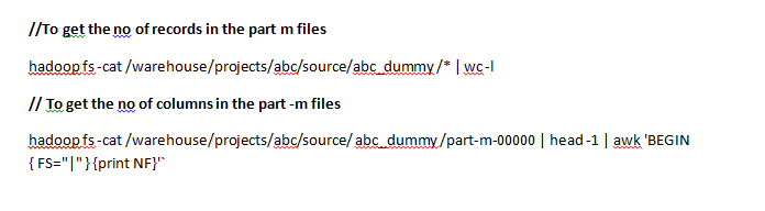
hadoop and hdfs commands


Counting the no of rows and columns in hadoop part-m files


Counting the no of rows and columns in hadoop part-m files:


Hive Alter Commands

Hive Alter Commands :


How To Extract JKS (Java KeyStore) from PEM file

How to Extract JKS (Java KeyStore) from PEM file 

The below steps has to be perfomed to extract jks from pem file

Step 1:
opensslx5O9 -outform der-in/bidata/projects/abc/keystore/cba.pem -out
/bidata/projects/abc/keystore/abcKeyStore.der

Step 2:
keytool-import-alias your-alias -keystore /bidata/projects/abc/keystore/abcKeystore.ks -file
/bidata/projetfs/abc/keystore/abcKeyStore.der


Tuesday, 27 December 2016

Unix Shell Scripting Commands - Part 1

Unix Shell Scripting :

We interact with the Unix kernel with the help shell application (which is called Terminal)
All unix commands have to be in lower case.

clear : clears the screen

cd ~ : Navigate to root folder

who am I : displays  three colums ( username, terminal id, time and date of login)

pwd  : shows the directory where the shell is in.  (pwd stands for present working directory)

cal : shows the calendar of the current month and year and current date is highlighted

cal 8 2007 or cal aug 2007 : calendar of august 2007 will be displayed

date : displays the date ( displays in default format)

To display date in custom format , then we do in the following way
date  ‘+DATE: %m-%y%Ntime:%H%M%S’ :
if you observe in the above command we have written in capital letters, that is not a command,that is to define format , so it can be written in capital letters

touch file1 file2  : this commands creates files in home directory

mkdir testdir :  creates a directory with name testdir in the home directory

mkdir documents/testdir : creates a directory in the documents path

cd testdir : changes the present working directory to the testdir , to create a file and content

cat > test : write the contents of the file, ctrl + D to end the editing

cat < test : to show the contents of the file.

Merge two files  cat > file1 file2 > file3  : contents of file1 and file2 will be merged and copied into file3

Rename and Delete :
mv oldfilename newfilename  : this renames the file or dire to new name given
rm filename : file will be deleted
rm –r directoryname  :  to deleted the directory
rmdir directoryname : also deleted the directory

Copies :
cp file_to_be_copied  destinationpath  : copies the file to the destination path
Links
   Hardlinks : creates a replica : ln old new :
   Softlinks : create a shortcut

File Permissions :
Every file or directory have below types of permissions
Owner
Read/Write
Group having access
Others

umask :  displays the four digit no , ignore the first digit , and substract the number from 666 if it is a file and from 777 if it is a directory,
ex : if the value 0022 for a file, subtract the value from 666 which give 644, that means the owner has read and write permissions where as the group and others have just read access.

chmod :  is used to modify file permissions of a file or directory
   ex : chmod 666 filename   : gives read and write to all for a file

Contents of directory:
      ls : lists the folders and files in a file of the home directory
       ls directoryname : 
       ls - l : longlist .
       ls – a : lists all the files along with hidden files
        file * : displays the contents of the folder, says the type of file ,directory etc
        ls –ltra  (shows all the hidden files
       ls –F : helps us to differentiate between files and directories

   
OS version details
uname –a : to now the version of the os and 

Count characters, words and lines:
1.wc filenametobeevaluated : displays the no of lines, words and characters
2.wc –l filenametobeevaluated :If we want only no of line then simply use
    

Sorting :
sort filetobesorted : the lines in the file will be sorted


Spark Memory Management

 Spark’s performance advantage over MapReduce  is due to Spark’s In-Memory Persistence and Memory Management Rather than writing to disk ...